Applied Mathematics

Math Modeling in Indudustry Team 7 - Intrim Report

Speaker: 
Matthew Hassell
Date: 
Mon, Aug 11, 2014
Location: 
PIMS, University of British Columbia
Conference: 
IMA-PIMS Math Modeling in Industry Workshop
Abstract: 

TBA

Class: 

Math Modeling in Indudustry Team 6 - Intrim Report

Speaker: 
Nathaniel Richmond
Date: 
Mon, Aug 11, 2014
Location: 
PIMS, University of British Columbia
Conference: 
IMA-PIMS Math Modeling in Industry Workshop
Abstract: 

TBA
 

Class: 

Math Modeling in Indudustry Team 4 - Intrim Report

Speaker: 
Jeremy Chiu
Date: 
Mon, Aug 11, 2014
Location: 
PIMS, University of British Columbia
Conference: 
IMA-PIMS Math Modeling in Industry Workshop
Abstract: 

TBA

Class: 

Math Modeling in Indudustry Team 3 - Intrim Report

Speaker: 
Timothy Costa
Date: 
Mon, Aug 11, 2014
Location: 
PIMS, University of British Columbia
Conference: 
IMA-PIMS Math Modeling in Industry Workshop
Abstract: 

TBA

Class: 

Math Modeling in Indudustry Team 2 - Intrim Report

Speaker: 
Brian Goddard
Alejandra Herrera Reyes
Date: 
Mon, Aug 11, 2014
Location: 
PIMS, University of British Columbia
Conference: 
IMA-PIMS Math Modeling in Industry Workshop
Abstract: 

TBA

Class: 

Math Modeling in Indudustry Team 7

Speaker: 
Tom Hogan
Date: 
Tue, Aug 5, 2014
Location: 
PIMS, University of British Columbia
Conference: 
IMA-PIMS Math Modeling in Industry Workshop
Abstract: 

Geometry (e.g., curves, surfaces, solids) is pervasive throughout the airplane industry.  At The Boeing Company, the prevalent way to model geometry is the parametric representation. For example, a parametric surface, S, is the image of a function

S:D → ℝ³

where D ≔ [0..1]×[0..1] is the parameter domain.

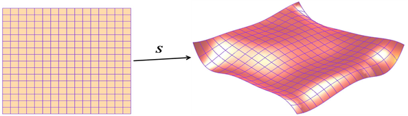
Here S denotes the parametrization, as well as the (red) surface itself.

A geometry’s parametric representation is not unique and the accuracy of analysis tools is often sensitive to its quality.  In many cases, the best parametrization is one that preserves lengths, areas, and angles well, i.e., a parametrization that is nearly isometric.  Nearly isometric parametrizations are used, for example, when designing non-flat parts that will be constructed or machined flat.

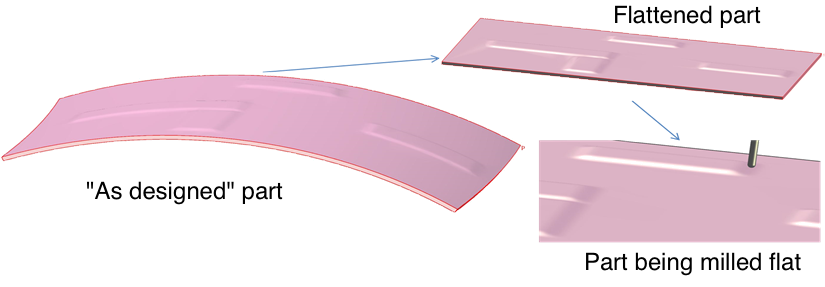
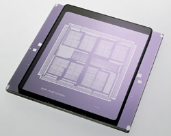
Figure 1. Parts that are nearly developable on one side are often machined on a flat table; then re-formed.

Another area where geometry parametrization is especially important is shape optimization activities that involve isogeometric analysis.  In these cases, getting a “good enough” parametrization very efficiently is crucial, since the geometry varies from one iteration to another. 

In this project, the students will research, discuss, and propose potential measures of “isometricness” and algorithms for obtaining them.  Example problems will be available on which to test their ideas.

References
1.    Michael S. Floater, Kai Hormann, Surface parametrization: a tutorial and survey, Advances in Multiresolution for Geometric Modeling, (2005) pp 157—186.
2.    J. Gravesen, A. Evgrafov, Dang-Manh Nguyen, P.N. Nielsen, Planar parametrization in isogeometric analysis, Lecture Notes in Computer Science, Volume 8177 (2014) pp 189—212.
3.    T-C Lim, S. Ramakrishna, Modeling of composite sheet forming: a review, Composites: Part A, Volume 33 (2002) pp 515—537.
4.    Yaron Lipman, Ingrid Daubechies, Conformal Wasserstein distances: comparing surfaces in polynomial time, Advances in Mathematics, vol. 227 (2010) pp. 1047—1077.

Class: 

Math Modeling in Indudustry Team 6

Speaker: 
Albert Gilg
Date: 
Tue, Aug 5, 2014
Location: 
PIMS, University of British Columbia
Conference: 
IMA-PIMS Math Modeling in Industry Workshop
Abstract: 

In real-life applications critical areas are often non- accessible for measurement and thus for inspection and control. For proper and safe operations one has to estimate their condition and predict their future alteration via inverse problem methods based on accessible data. Typically such situations are even complicated by unreliable or flawed data such as sensor data rising questions of reliability of model results. We will analyze and mathematically tackle such problems starting with physical vs. data driven modeling, numerical treatment of inverse problems, extension to stochastic models and statistical approaches to gain stochastic distributions and confidence intervals for safety critical parameters.

As project example we consider a blast furnace producing iron at temperatures around 2,000 °C. It is running several years without stop or any opportunity to inspect its inner geometry coated with firebrick. Its inner wall is aggressively penetrated by physical and chemical processes. Thickness of the wall, in particular evolvement of weak spots through wall thinning is extremely safety critical. The only available data stem from temperature sensors at the outer furnace surface. They have to be used to calculate wall thickness and its future alteration. We will address some of the numerous design and engineering questions such as placement of sensors, impact of sensor imprecision and failure.

References:
1. F. Bornemann, P. Deuflhard, A. Hohmann, "Numerical Analysis”, de Gruyter, 1995
2. A. C. Davison,” Statistical Models”, Cambridge University Press, 2003
3. William H. Press, “Numerical Recipes in C”, Cambridge University Press, 1992
4. http://en.wikipedia.org/wiki/Blast_furnace#Modern_process
Prerequisites:
Computer programming experience in a language like C or C++; Knowledge about Numerical Linear Algebra,
Stochastic and Statistics (see references)

Class: 

Math Modeling in Indudustry Team 4

Speaker: 
Dimitar Trenev
Date: 
Tue, Aug 5, 2014
Location: 
PIMS, University of British Columbia
Conference: 
IMA-PIMS Math Modeling in Industry Workshop
Abstract: 

Linear systems of saddle-point type arise in a range of applications including optimization, mixed finite-element methods [1] for mechanics and fluid dynamics, economics, and finance. Due to their indefiniteness and generally unfavorable spectral properties, such systems are difficult to solve, particularly when their dimension is very large. In some applications - for example, when simulating fluid flow over large periods of time - such systems have to be solved many times over the course of a single run, and the linear solver rapidly becomes a major bottleneck. For this reason, finding an efficient and scalable solver is of the utmost importance.

In this project, participants will be asked to propose and examine various solution strategies for saddle-point systems (see [2] for a very good, if slightly dated, survey). They will test the performance of those strategies on simple systems modeling flows in porous media. The different strategies will then be ranked based on their applicability, efficiency, and robustness.

Some knowledge of linear algebra and the basics of iterative solvers is expected. Familiarity with MATLAB is necessary.

References

[1] F. Brezzi and M. Fortin, Mixed and hybrid finite element methods, New York, Springer-Verlag, 1991.

[2] M. Benzi, G. H. Golub, J. Liesen, Numerical solution of saddle point problems, Acta Numerica (14), pp. 1-137, Cambridge University Press, 2005.

Class: 

Math Modeling in Indudustry Team 3

Speaker: 
Apo Sezginer
Date: 
Tue, Aug 5, 2014
Location: 
PIMS, University of British Columbia
Conference: 
IMA-PIMS Math Modeling in Industry Workshop
Abstract: 

Integrated circuits are manufactured by optical projection lithography.  The circuit pattern is etched on a master copy, the photomask.  Light is projected through the photomask and its image is formed on the semiconductor wafer under production.  The image is transferred to the integrated circuit by a photographic process.  On the order of 40 lithography steps are needed to produce an integrated circuit.   Most advanced lithography is performed using the 193 nm ArF excimer wavelength, about three times smaller than the wavelength of visible red light.  Critical dimensions of the circuit pattern are smaller than the wavelength of the projected light.  Sub-wavelength resolution is achieved by optical resolution enhancement techniques and the non-linearity of the chemistry. 

Calculating the optical image accurately and rapidly is required for two reasons: first the design of the photomask is an inverse problem.  A good forward solution is needed to solve the inverse problem iteratively.  Second, the photomask is inspected by a microscope to find manufacturing defects.  The correct microscope image is calculated, and the actual microscope image is compared to the calculated reference image to find defects.  The most significant part of the image calculation is the diffraction of the illuminating wave by the photomask.  Although rigorous solution of Maxwell's Equations by numerical methods is well known, either the speed or the accuracy of known methods is not satisfactory.  The most commonly used method is Kirchhoff approximation amended by some fudge factors to make it closer to the rigorous solution. 

Kirchhoff solved the problem diffraction of light through an arbitrarily shaped aperture in an opaque screen at the end of 19th century.  He had a very practical approximation for the near-field of the screen, on the side that is opposite to the light source.  At a point on the screen, he ignored that there is an aperture.  At a point at the aperture, he ignored that there is a screen.  He used Green's theorem to propagate this estimate of the near-field to the far-field.  Kirchhoff’s near-field approximation is accurate for points that are a few wave-lengths away from the edges.   The Kirchhoff near-field is discontinuous at the edges and it violates boundary conditions for Maxwell’s Equations.  To this day an amended form of Kirchhoff’s approximation provides the best known accuracy-speed trade-off to calculate the image of a photomask.

The Goal of this Project

We will attempt to improve the accuracy of the Kirchhoff’s approximation.  We will cast Maxwell’s Equations into a linear matrix equation Ax=b where x is a vector of electric and magnetic field values.  This can be done either using finite differences or using a weak (integral) form of Maxwell’s Equations.  We will initialize the vector x with the Kirchhoff solution.  We will use an iterative linear equation solver such as GMRES.  The goal is to improve the solution in very few iterations.

Class: 

Intermediary Leverage Cycles and Financial Stability

Author: 
Tobias Adrian
Date: 
Wed, Jul 30, 2014
Location: 
PIMS, University of British Columbia
Conference: 
PIMS Workshop on the Economics and Mathematics of Systemic Risk
Abstract: 

We present a theory of financial intermediary leverage cycles within a dynamic model of the macroeconomy. Intermediaries face risk-based funding constraints that give rise to procyclical leverage and a procyclical share of intermediated credit. The pricing of risk varies as a function of intermediary leverage, and asset return exposure to intermediary leverage shocks earns a positive risk premium. Relative to an economy with constant leverage, financial intermediaries generate higher consumption growth and lower consumption volatility in normal times, at the cost of endogenous systemic financial risk. The severity of systemic crisis depends on intermediaries’ leverage and net worth. Regulations that tighten funding constraints affect the systemic risk-return trade-off by lowering the likelihood of systemic crises at the cost of higher pricing of risk. (Joint work with Nina Boyarchenko - FRBNY)

Class: 

Pages